Machine learning classifier

library(cyCONDOR)
library(ggplot2)
library(CytoDx)

With cyCONDOR we developed a set of functions allowing the user to easily train a classifier for the sample labels. In this vignette we exemplify all the steps required for the classification of AML (acute myeloid leukemia) and control samples. The trained model can then be used to predict the label of and external sample. This workflow is based on the CytoDX package, for detailed documentation see the original manuscript Hu et. al, 2019, Bioinformatics and cytoDXdocumentation of Bioconductor.

We will start the vignette by loading a training dataset, in this dataset the clinical classification of the sample is known and will be used to train a cytoDX model. In cyCONDOR the cytoDX model is saved withing the condor object and can be used to classify new samples.

If you use this workflow in your work please consider citing cyCONDOR and cytoDX.

Train the `cytoDX` model

Load the data

We start by importing the training dataset, this is done as previously described with the prep_fcd function, in this case the anno_table also include the clinical classification of the samples (aml or normal).

condor <- prep_fcd(data_path = "../.test_files/ClinicalClassifier/train/", 
                   max_cell = 10000000, 
                   useCSV = FALSE, 
                   transformation = "auto_logi", 
                   remove_param = c("FSC-A","FSC-W","FSC-H","Time"), 
                   anno_table = "../.test_files/ClinicalClassifier/fcs_info_train.csv", 
                   filename_col = "fcsName",
                   seed = 91)

Build the classifier model

We now train the cytoDX classifier on the sample label, this step does not require any other pre-analysis on the dataset, nevertheless, if you are not familiar with the data you are using for training we recommend an exploratory data analysis first.

# Re order variables - this is not strictly needed but the classification always consider the first variable as reference.

condor$anno$cell_anno$Label <- factor(condor$anno$cell_anno$Label, 
                                      levels = c("normal", "aml"), 
                                      labels = c("1_normal", "2_aml"))

The train_classifier_model requires the user to define the input table and few parameter to be used for training the cytoDX model. As some of the variables are derived from the cytoDX package (cytoDX.fit function) please refer to cytoDX documentation for further details.

fcd: Flow cytometry data set to be used for training the model.
input_type: data slot to be used for the classification, suggested expr.
data slot: exact name of the data slot to be used (orig or norm, if batch correction was performed).
sample_names: name of the column of the anno_table containing the sample names.
classification_variable: name of the column of the anno_table containing the clinical classification to be used for training the classifier.
type1: type of first level prediction, parameter inherited from cytoDX, see cytoDX documentation for details.
type2: type of second level prediction, parameter inherited from cytoDX, see cytoDX documentation for details.
parallelCore: number of cores to be used.

condor <- train_classifier_model(fcd = condor, 
                                 input_type = "expr", 
                                 data_slot = "orig", 
                                 sample_names = "expfcs_filename", 
                                 classification_variable = condor$anno$cell_anno$Label, 
                                 family = "binomial", 
                                 type1 = "response", 
                                 parallelCore = 1, 
                                 reg = FALSE, 
                                 seed = 91)

## Warning in lognet(x, is.sparse, y, weights, offset, alpha, nobs, nvars, : one
## multinomial or binomial class has fewer than 8 observations; dangerous ground

Explore the result of model training

We can now explore the results of the cell level and sample level prediction on the training data. The results are stored together with the cytoDX model itself in the extras slot (classifier_model)

Cell level predition result on the training dataset

The cellular level result contain the probability of classification to aml for each cell in the dataset, this table also include the true label of each cell.

head(condor$extras$classifier_model$train.Data.cell)

##         sample y1.Truth y.Pred.s0
## 1 sample11.fcs    2_aml 0.5836773
## 2 sample11.fcs    2_aml 0.5299637
## 3 sample11.fcs    2_aml 0.6896542
## 4 sample11.fcs    2_aml 0.4914881
## 5 sample11.fcs    2_aml 0.5393115
## 6 sample11.fcs    2_aml 0.3407959

Sample level predition result on the training dataset

The sample level result contain the probability of classification to aml for each cell in the dataset, this table also include the true label of each cell.

head(condor$extras$classifier_model$train.Data.sample)

##                    sample y1.Truth    y.Pred.s0
## sample11.fcs sample11.fcs    2_aml 1.000000e+00
## sample12.fcs sample12.fcs    2_aml 1.000000e+00
## sample13.fcs sample13.fcs    2_aml 9.999999e-01
## sample14.fcs sample14.fcs    2_aml 1.000000e+00
## sample15.fcs sample15.fcs    2_aml 1.000000e+00
## sample16.fcs sample16.fcs 1_normal 5.949578e-14

Visualize the results on the train dataset

We can now visualize the prediction result both at cell and sample level.

anno <- read.csv("../.test_files/ClinicalClassifier/fcs_info_train.csv")

ggplot(merge(x = condor$extras$classifier_model$train.Data.cell, y = anno, by.x = "sample", by.y = "fcsName"), aes(x = sample, y = y.Pred.s0, color = Label)) +
  geom_jitter() + 
  geom_violin() +
  scale_color_manual(values = c("#92278F", "#F15A29")) +
  theme_bw() + 
  theme(aspect.ratio = 1) + 
  ylab("probability") + 
  ggtitle("sample level prediction - train data") + 
  theme(axis.text.x = element_text(angle = 45, hjust = 1))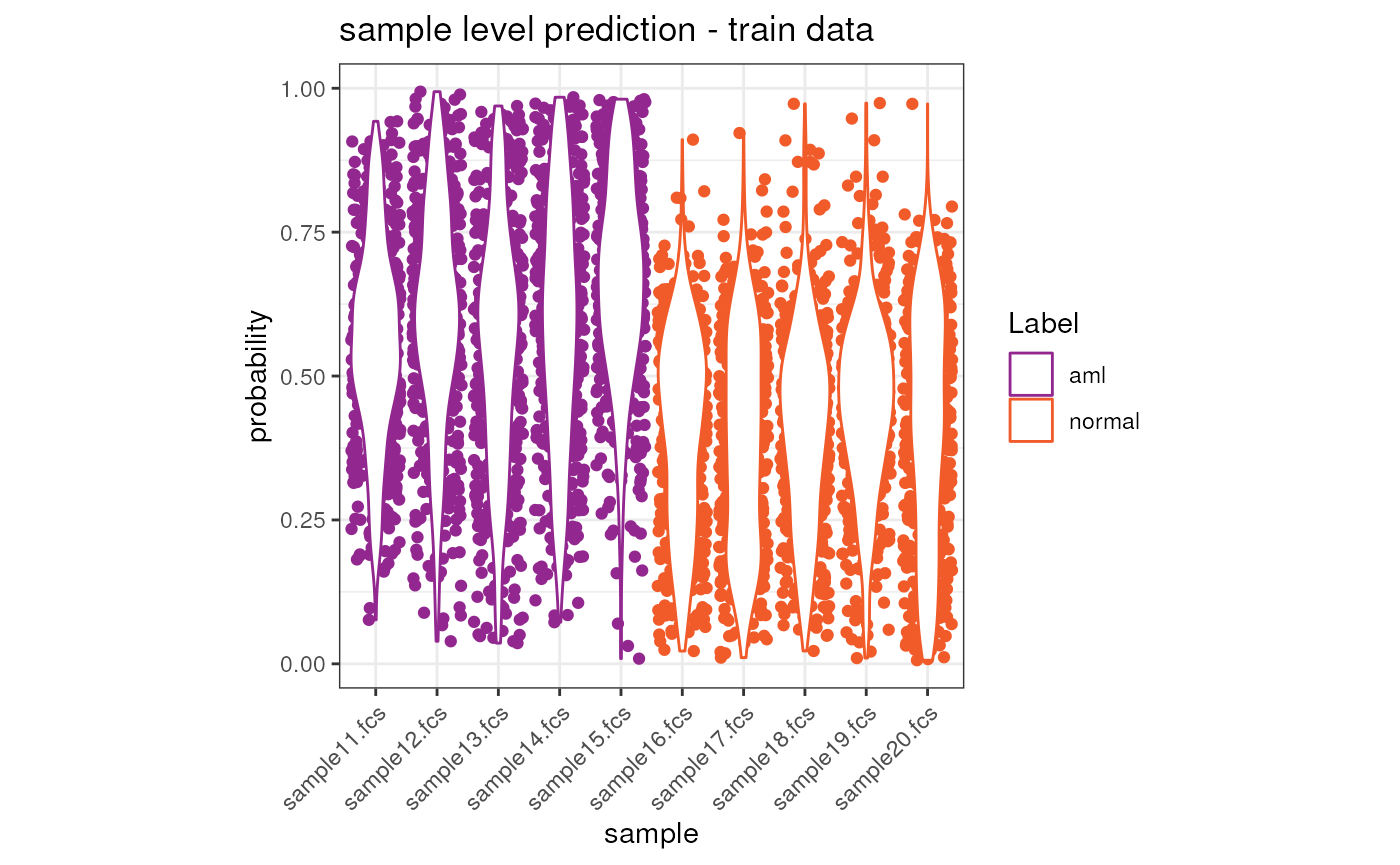

ggplot(merge(x = condor$extras$classifier_model$train.Data.sample, y = anno, by.x = "sample", by.y = "fcsName"), aes(x = sample, y = y.Pred.s0, color = Label)) +
  geom_point(size = 4) +
  scale_color_manual(values = c("#92278F", "#F15A29")) +
  theme_bw() + 
  theme(aspect.ratio = 2) + 
  ylab("probability") +
  ggtitle("sample level prediction - train data") + 
  theme(axis.text.x = element_text(angle = 45, hjust = 1))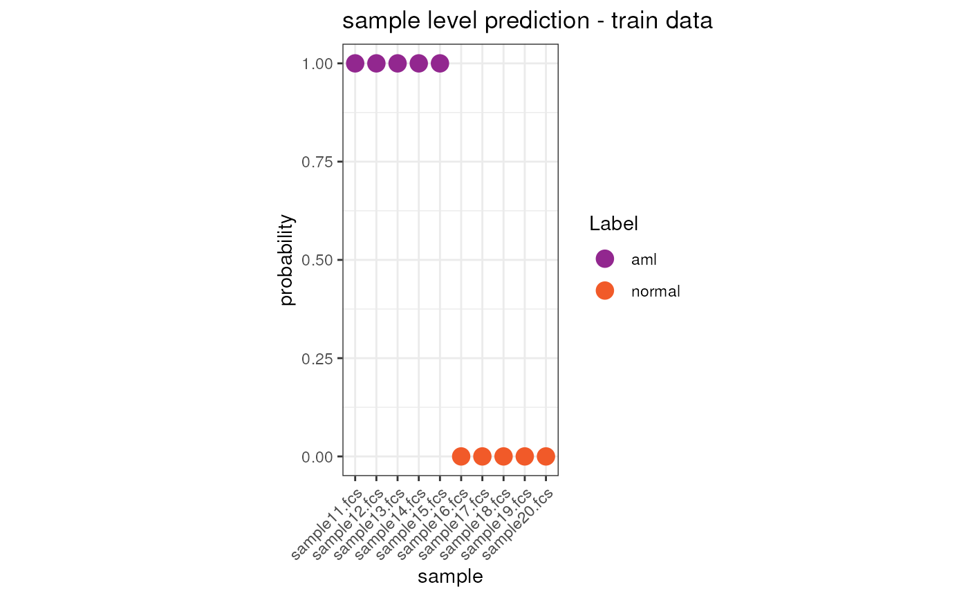

Visualization of the decision tree

We can use a cytoDX built-in function to visualize the decision tree used for the cell level classification. See cytoDX documentation for further details.

tree <- treeGate(P = condor$extras$classifier_model$train.Data.cell$y.Pred.s0,
                 x= condor$expr$orig)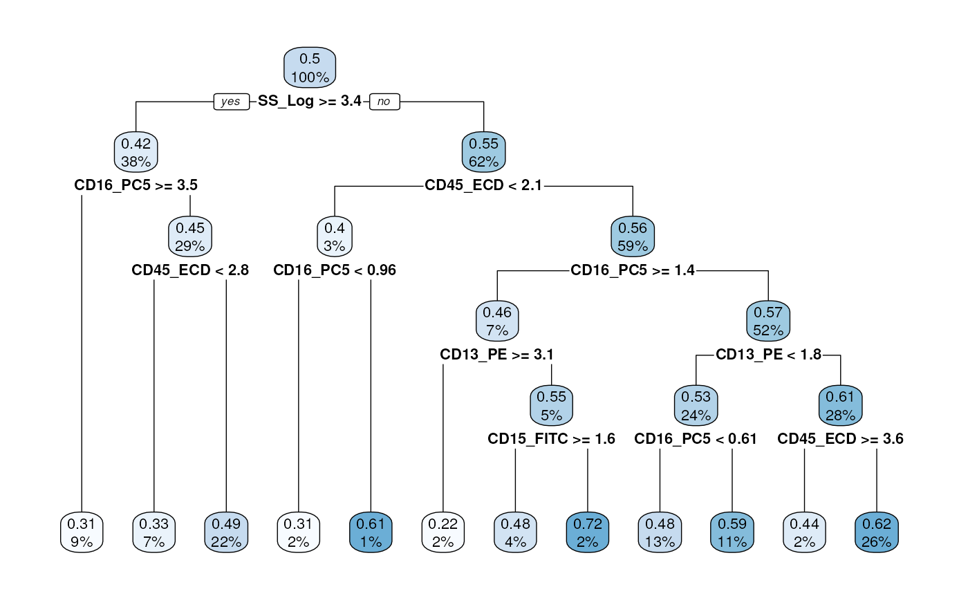

Testing on an independent dataset

Load the data

To now validate the performance of the trained cytoDX model we will test it on a test dataset with no overlap with the training data.

condor_test <- prep_fcd(data_path = "../.test_files/ClinicalClassifier/test/", 
                        max_cell = 10000000, 
                        useCSV = FALSE, 
                        transformation = "auto_logi", 
                        remove_param = c("FSC-A","FSC-W","FSC-H","Time"), 
                        anno_table = "../.test_files/ClinicalClassifier/fcs_info_test.csv", 
                        filename_col = "fcsName",
                        seed = 91)

Predict classification

We can now predict the label using the trained model

# Re order variables - this is not strictly needed but the classification always consider the first variable as reference.

condor_test$anno$cell_anno$Label <- factor(condor_test$anno$cell_anno$Label, 
                                           levels = c("normal", "aml"), 
                                           labels = c("1_normal", "2_aml"))

The predict_classifier requires few user defined input to predict the labels of an external dataset using a previously prepared cytoDX model.

fcd: flow cytometri dataset of the new data
input_type: data slot to be used for the classification, suggested expr. Should match the option selection in train_classifier_model.
data slot: exact name of the data slot to be used (orig or norm, if batch correction was performed). Should match the option selection in train_classifier_model.
sample_names: name of the column in the anno_table containing the sample names.
model_object: cyCONDOR trained cytoDX model, this is stored in the condor object used to train the model (extras slot).

condor_test <- predict_classifier(fcd = condor_test, 
                                  input_type = "expr", 
                                  data_slot = "orig", 
                                  sample_names = "expfcs_filename", 
                                  model_object = condor$extras$classifier_model, 
                                  seed = 91)

Explore the result of prediction in test dataset

We can now explore the results of the cell level and sample level prediction on the test data. The results are stored together with the cytoDX model itself in the extras slot (classifier_prediction)

Cell level predition result on the test dataset

The cellular level result contain the probability of classification to aml for each cell in the dataset.

head(condor_test$extras$classifier_prediction$xNew.Pred.cell)

##        sample y.Pred.s0
## 1 sample1.fcs 0.6212374
## 2 sample1.fcs 0.6780328
## 3 sample1.fcs 0.5818562
## 4 sample1.fcs 0.3354043
## 5 sample1.fcs 0.4015879
## 6 sample1.fcs 0.7143018

Cell level predition result on the test dataset

The sample level result contain the probability of classification to aml for each cell in the dataset.

head(condor_test$extras$classifier_prediction$xNew.Pred.sample)

##                    sample    y.Pred.s0
## sample1.fcs   sample1.fcs 1.000000e+00
## sample10.fcs sample10.fcs 6.021657e-12
## sample2.fcs   sample2.fcs 1.000000e+00
## sample3.fcs   sample3.fcs 9.998114e-01
## sample4.fcs   sample4.fcs 1.000000e+00
## sample5.fcs   sample5.fcs 1.000000e+00

Visualize the results on the test dataset

We can now visualize the prediction result both at cell and sample level.

anno <- read.csv("../.test_files/ClinicalClassifier/fcs_info_test.csv")

tmp <- merge(x = condor_test$extras$classifier_prediction$xNew.Pred.cell, y = anno, by.x = "sample", by.y = "fcsName")

tmp$sample <- factor(tmp$sample, levels = c("sample1.fcs", "sample2.fcs", "sample3.fcs",  "sample4.fcs",  "sample5.fcs",  "sample6.fcs",  "sample7.fcs",  "sample8.fcs",  "sample9.fcs", "sample10.fcs"))

ggplot(tmp, aes(x = sample, y = y.Pred.s0, color = Label)) +
  geom_jitter() +
  geom_violin() +
  scale_color_manual(values = c("#92278F", "#F15A29")) +
  theme_bw() + 
  theme(aspect.ratio = 1) + 
  ylab("probability") +
  ggtitle("cell level prediction - test data") + 
  theme(axis.text.x = element_text(angle = 45, hjust = 1))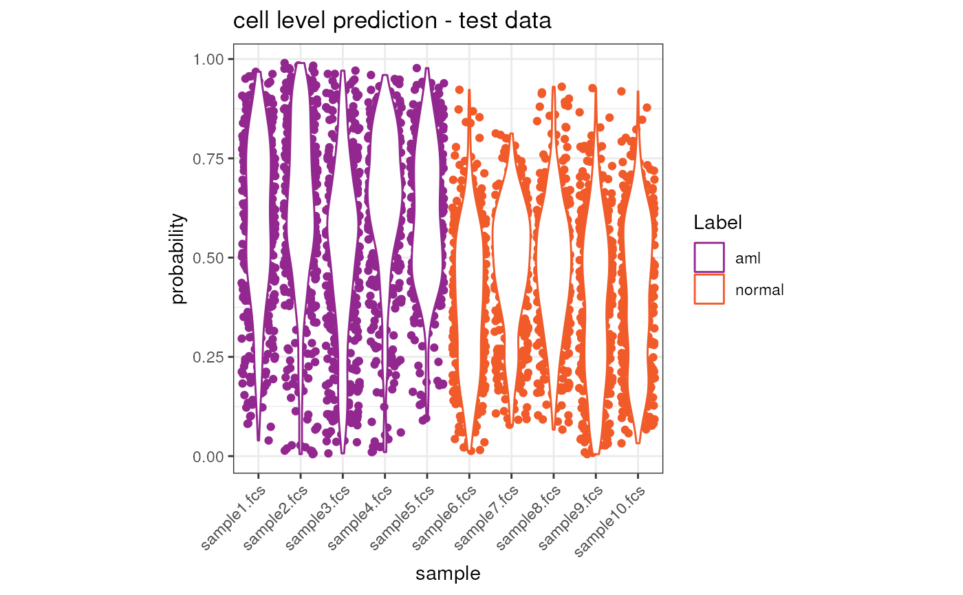

rm(tmp)

tmp <- merge(x = condor_test$extras$classifier_prediction$xNew.Pred.sample, y = anno, by.x = "sample", by.y = "fcsName")

tmp$sample <- factor(tmp$sample, levels = c("sample1.fcs", "sample2.fcs", "sample3.fcs",  "sample4.fcs",  "sample5.fcs",  "sample6.fcs",  "sample7.fcs",  "sample8.fcs",  "sample9.fcs", "sample10.fcs"))

ggplot(tmp, aes(x = sample, y = y.Pred.s0, color = Label)) +
  geom_point(size = 4) +
  scale_color_manual(values = c("#92278F", "#F15A29")) +
  theme_bw() + 
  theme(aspect.ratio = 2) + 
  ylab("probability") +
  ggtitle("sample level prediction - test data") + 
  theme(axis.text.x = element_text(angle = 45, hjust = 1))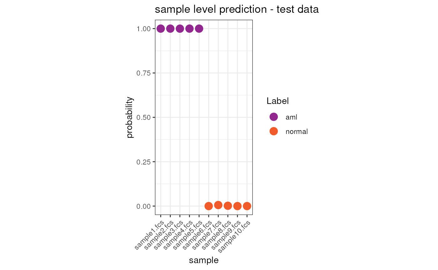

rm(tmp)

Session Info

info <- sessionInfo()

info

## R version 4.4.2 (2024-10-31)
## Platform: x86_64-pc-linux-gnu
## Running under: Ubuntu 24.04.1 LTS
## 
## Matrix products: default
## BLAS:   /usr/lib/x86_64-linux-gnu/openblas-pthread/libblas.so.3 
## LAPACK: /usr/lib/x86_64-linux-gnu/openblas-pthread/libopenblasp-r0.3.26.so;  LAPACK version 3.12.0
## 
## locale:
##  [1] LC_CTYPE=en_US.UTF-8       LC_NUMERIC=C              
##  [3] LC_TIME=en_US.UTF-8        LC_COLLATE=en_US.UTF-8    
##  [5] LC_MONETARY=en_US.UTF-8    LC_MESSAGES=en_US.UTF-8   
##  [7] LC_PAPER=en_US.UTF-8       LC_NAME=C                 
##  [9] LC_ADDRESS=C               LC_TELEPHONE=C            
## [11] LC_MEASUREMENT=en_US.UTF-8 LC_IDENTIFICATION=C       
## 
## time zone: Etc/UTC
## tzcode source: system (glibc)
## 
## attached base packages:
## [1] stats     graphics  grDevices utils     datasets  methods   base     
## 
## other attached packages:
## [1] CytoDx_1.26.0  ggplot2_3.5.2  cyCONDOR_0.3.1
## 
## loaded via a namespace (and not attached):
##   [1] IRanges_2.40.1              Rmisc_1.5.1                
##   [3] urlchecker_1.0.1            nnet_7.3-20                
##   [5] CytoNorm_2.0.1              TH.data_1.1-3              
##   [7] vctrs_0.6.5                 digest_0.6.37              
##   [9] png_0.1-8                   shape_1.4.6.1              
##  [11] proxy_0.4-27                slingshot_2.14.0           
##  [13] ggrepel_0.9.6               corrplot_0.95              
##  [15] parallelly_1.45.0           MASS_7.3-65                
##  [17] pkgdown_2.1.3               reshape2_1.4.4             
##  [19] httpuv_1.6.16               foreach_1.5.2              
##  [21] BiocGenerics_0.52.0         withr_3.0.2                
##  [23] ggrastr_1.0.2               xfun_0.52                  
##  [25] ggpubr_0.6.1                ellipsis_0.3.2             
##  [27] survival_3.8-3              memoise_2.0.1              
##  [29] hexbin_1.28.5               ggbeeswarm_0.7.2           
##  [31] RProtoBufLib_2.18.0         princurve_2.1.6            
##  [33] profvis_0.4.0               ggsci_3.2.0                
##  [35] systemfonts_1.2.3           ragg_1.4.0                 
##  [37] zoo_1.8-14                  GlobalOptions_0.1.2        
##  [39] DEoptimR_1.1-3-1            Formula_1.2-5              
##  [41] promises_1.3.3              scatterplot3d_0.3-44       
##  [43] httr_1.4.7                  rstatix_0.7.2              
##  [45] globals_0.18.0              rstudioapi_0.17.1          
##  [47] UCSC.utils_1.2.0            miniUI_0.1.2               
##  [49] generics_0.1.4              ggcyto_1.34.0              
##  [51] base64enc_0.1-3             curl_6.4.0                 
##  [53] S4Vectors_0.44.0            zlibbioc_1.52.0            
##  [55] flowWorkspace_4.18.1        polyclip_1.10-7            
##  [57] randomForest_4.7-1.2        GenomeInfoDbData_1.2.13    
##  [59] SparseArray_1.6.2           RBGL_1.82.0                
##  [61] ncdfFlow_2.52.1             RcppEigen_0.3.4.0.2        
##  [63] xtable_1.8-4                stringr_1.5.1              
##  [65] desc_1.4.3                  doParallel_1.0.17          
##  [67] evaluate_1.0.4              S4Arrays_1.6.0             
##  [69] hms_1.1.3                   glmnet_4.1-9               
##  [71] GenomicRanges_1.58.0        irlba_2.3.5.1              
##  [73] colorspace_2.1-1            harmony_1.2.3              
##  [75] reticulate_1.42.0           readxl_1.4.5               
##  [77] magrittr_2.0.3              lmtest_0.9-40              
##  [79] readr_2.1.5                 Rgraphviz_2.50.0           
##  [81] later_1.4.2                 lattice_0.22-7             
##  [83] future.apply_1.20.0         robustbase_0.99-4-1        
##  [85] XML_3.99-0.18               cowplot_1.2.0              
##  [87] matrixStats_1.5.0           xts_0.14.1                 
##  [89] class_7.3-23                Hmisc_5.2-3                
##  [91] pillar_1.11.0               nlme_3.1-168               
##  [93] iterators_1.0.14            compiler_4.4.2             
##  [95] RSpectra_0.16-2             stringi_1.8.7              
##  [97] gower_1.0.2                 minqa_1.2.8                
##  [99] SummarizedExperiment_1.36.0 lubridate_1.9.4            
## [101] devtools_2.4.5              CytoML_2.18.3              
## [103] plyr_1.8.9                  crayon_1.5.3               
## [105] abind_1.4-8                 locfit_1.5-9.12            
## [107] sp_2.2-0                    sandwich_3.1-1             
## [109] pcaMethods_1.98.0           dplyr_1.1.4                
## [111] codetools_0.2-20            multcomp_1.4-28            
## [113] textshaping_1.0.1           recipes_1.3.1              
## [115] openssl_2.3.3               Rphenograph_0.99.1         
## [117] TTR_0.24.4                  bslib_0.9.0                
## [119] e1071_1.7-16                destiny_3.20.0             
## [121] GetoptLong_1.0.5            ggplot.multistats_1.0.1    
## [123] mime_0.13                   splines_4.4.2              
## [125] circlize_0.4.16             Rcpp_1.1.0                 
## [127] sparseMatrixStats_1.18.0    cellranger_1.1.0           
## [129] knitr_1.50                  clue_0.3-66                
## [131] lme4_1.1-37                 fs_1.6.6                   
## [133] listenv_0.9.1               checkmate_2.3.2            
## [135] DelayedMatrixStats_1.28.1   Rdpack_2.6.4               
## [137] pkgbuild_1.4.8              ggsignif_0.6.4             
## [139] tibble_3.3.0                Matrix_1.7-3               
## [141] rpart.plot_3.1.2            statmod_1.5.0              
## [143] tzdb_0.5.0                  tweenr_2.0.3               
## [145] pkgconfig_2.0.3             pheatmap_1.0.13            
## [147] tools_4.4.2                 cachem_1.1.0               
## [149] rbibutils_2.3               smoother_1.3               
## [151] fastmap_1.2.0               rmarkdown_2.29             
## [153] scales_1.4.0                grid_4.4.2                 
## [155] usethis_3.1.0               broom_1.0.8                
## [157] sass_0.4.10                 graph_1.84.1               
## [159] carData_3.0-5               RANN_2.6.2                 
## [161] rpart_4.1.24                farver_2.1.2               
## [163] reformulas_0.4.1            yaml_2.3.10                
## [165] MatrixGenerics_1.18.1       foreign_0.8-90             
## [167] ggthemes_5.1.0              cli_3.6.5                  
## [169] purrr_1.1.0                 stats4_4.4.2               
## [171] lifecycle_1.0.4             uwot_0.2.3                 
## [173] askpass_1.2.1               caret_7.0-1                
## [175] Biobase_2.66.0              mvtnorm_1.3-3              
## [177] lava_1.8.1                  sessioninfo_1.2.3          
## [179] backports_1.5.0             cytolib_2.18.2             
## [181] timechange_0.3.0            gtable_0.3.6               
## [183] rjson_0.2.23                umap_0.2.10.0              
## [185] ggridges_0.5.6              parallel_4.4.2             
## [187] pROC_1.18.5                 limma_3.62.2               
## [189] jsonlite_2.0.0              edgeR_4.4.2                
## [191] RcppHNSW_0.6.0              Rtsne_0.17                 
## [193] FlowSOM_2.14.0              ranger_0.17.0              
## [195] flowCore_2.18.0             jquerylib_0.1.4            
## [197] timeDate_4041.110           shiny_1.11.1               
## [199] ConsensusClusterPlus_1.70.0 htmltools_0.5.8.1          
## [201] diffcyt_1.26.1              glue_1.8.0                 
## [203] XVector_0.46.0              VIM_6.2.2                  
## [205] gridExtra_2.3               boot_1.3-31                
## [207] TrajectoryUtils_1.14.0      igraph_2.1.4               
## [209] R6_2.6.1                    tidyr_1.3.1                
## [211] SingleCellExperiment_1.28.1 labeling_0.4.3             
## [213] vcd_1.4-13                  cluster_2.1.8.1            
## [215] pkgload_1.4.0               GenomeInfoDb_1.42.3        
## [217] ipred_0.9-15                nloptr_2.2.1               
## [219] DelayedArray_0.32.0         tidyselect_1.2.1           
## [221] vipor_0.4.7                 htmlTable_2.4.3            
## [223] ggforce_0.5.0               car_3.1-3                  
## [225] future_1.58.0               ModelMetrics_1.2.2.2       
## [227] laeken_0.5.3                data.table_1.17.8          
## [229] htmlwidgets_1.6.4           ComplexHeatmap_2.22.0      
## [231] RColorBrewer_1.1-3          rlang_1.1.6                
## [233] remotes_2.5.0               colorRamps_2.3.4           
## [235] ggnewscale_0.5.2            hardhat_1.4.1              
## [237] beeswarm_0.4.0              prodlim_2025.04.28

Train the cytoDX model

Load the data

Build the classifier model

Explore the result of model training

Cell level predition result on the training dataset

Sample level predition result on the training dataset

Visualize the results on the train dataset

Visualization of the decision tree

Testing on an independent dataset

Load the data

Predict classification

Explore the result of prediction in test dataset

Cell level predition result on the test dataset

Cell level predition result on the test dataset

Visualize the results on the test dataset

Session Info

Train the `cytoDX` model